Disturbance Observer (DOB)

Robust Control Technique for parametric uncertainties, external disturbances, and unmodeled dynamics which preserves the relative degree of the system.

For this post, I’ll briefly introduce the Robust Control technique named Disturbance Observer(DOB). I first learned about DOB from ‘Advance Control Techniques’ class at SNU and realized that DOB has several attractive features.

Disturbance Observer(DOB) has demonstrated significant success in various industrial applications, owing to its robust capabilities to handle disturbances and model uncertainties. DOB serves as an add-on type inner-loop controller that makes the plant behaves just like a nominal plant, relieving the outer controller from the difficulties of addressing model uncertainties and disturbances. Imagine you already have your own controller for the specific system you’ve designed using the Nominal model.

But, how confident are you with the model you have?

Can you assert that your model fully represents your true system? This problem is particulary important for Safety Critial Systems(e.g., UAV, Robots, Autonomous Vehicles). In real world application, your true model may differ from your nominal model, and various factors contribute to this difference:

1. Parametric Uncertainties: Your model parameters, such as mass or length, might differ from your true system.
2. External Disturbances: For instance, your UAV might be affected by the wind while flying
3. Unmodeled Dynamics: Usually your model is designed using simplified dynamics(often linearized). The system’s dynamics, such as those inside the motors or the elasticity of the beam, are often ignored, which can easily change the system’s degree.

Basic Concept of DOB

Let’s first look at the following image. The image credit belongs to the Prof. Shim at SNU EE.

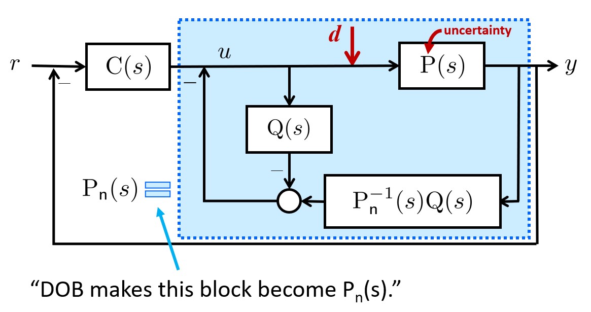
The goal of this control problem is to make your system output y to track the reference signal r under disturbance $d(t)$ and (parametric) uncertainty in the true system $P(s)$. The parametric uncertainty can also be understood that the coefficients of your transfer function is different between your nominal system and true system. Here, $P(s)$ is your true but unknown model, $C(s)$ is the controller, $P_n(s)$ is the known nominal model you have. $Q(s)$ is called ‘Q-filter’, plays a crucial role in the DOB.

By utilizing these structure, DOB makes the blue box behaves just like $P_n(s)$. This implies that the controller $C(s)$ can be designed using only the Nominal model without additional consideration. For example, imagine a simple control-system utilizing the linearized model, you might be concerned about using the simplified model might degrades the performances. In this case, you can “add” a DOB to your control system(without changing your controller) which makes your model behaves like your nominal model even under uncertainties and disturbances. For more information, you can check out some tutorial paper of DOB.

The condition to use the basic DOB structure is that the relative degree of the true and nominal systems need to be same. There were some advanced research which handles the problem when the relative degree changes, but we will not consider it for this post. Let the transfer function of the true system $P(s)$ be written as

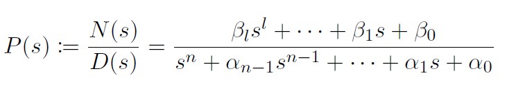
and the transfer function of the nominal system $P_n(s)$ be written as

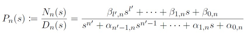
Here, let’s assume that the relative degree r is same for both true and nominal system, which indicates $r=n-l=n’-l’$.

Existing research papers commonly focus on cases where $n=n’$ and $l=l’$. However, I’ve found that when the relative degree remains consistent between the true and nominal systems, DOB can stabilize the system, irrespective of the system’s degree. Now, let the Q-filter with relative degree r as

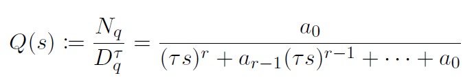
where tau determines the bandwidth of $Q(s)$. As $\tau$ becomes smaller, the performance of the DOB increases. Let the transfer function of the controller $C(s)$ as

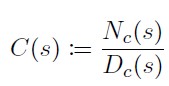
where degree of $N_c(s)$ is k, and degree of $D_c(s)$ is m.

Stability Condition for DOB

For this section, I’ll just give you the brief result of how we could make the DOB-based control system robustly stable. The characteristic polynomial of the closed-loop system can be written as

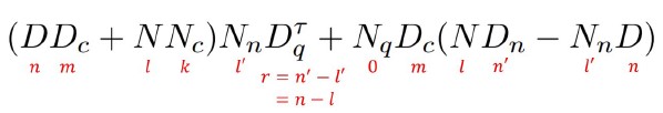
where the red number indicates the degree of each terms. From control theory, we know that the system is stable when all the roots of this characteristic polynomial have negative real part. Since directly obtaining the roots can be challenging, the behavior of the roots were analyzed when $\tau$ approaches to 0. This approach follows from this paper.

Roots of characteristic polynomial when tau approaches to zero

Lemma : As $\tau$ approach to 0,

• $n’+m+l$ number of roots aproach to the roots of
  • $N(s)(D_n(s)D_c(s)+N_n(s)N_c(s))$
• $n-l=r$ number of roots approach to the roots of
  • $p_f(s) = D_q^1(s) + (\frac{\beta_l}{\beta_{l’,n}}-1)N_q(s)$

Note that the unknown part of these equations are included in $N(s)$ and $\beta_l$. By utilizing these results, the stability condition could be denoted as following

DOB-Based control is robustly stable when the bandwidth of Q-filter is sufficiently large if

1. True plant is Minimum phase, and
2. $C(s)$ internally stabilizes $P_n(s)$, and
3. $p_f(s)$ is Hurwitz for all $\beta_l$

For those who are unfamiliar with the term “Minimum phase”, it indicates that the numerator(zeros) of your true transfer function is stable. When designing the Q-filter for the DOB, it is crucial to ensure that both your Q-filter and controller meet the conditions mentioned above. If you are interested in the Q-filter design for DOB implementation, numerous research papers are available online.

Conclusion

Despite omitting most of the proofs, I hope you get the concept of the DOB through this post. DOB proves effective in managing parametric uncertainties, external disturbances, and unmodeled dynamics when the relative degree remains the same(between true and nominal system).

While this post introduces DOB solely through frequency domain analysis, state-space analysis is also available. State-space analysis provides insights into the functionality of each component of DOB and aids in handling different extensions of DOB, such as MIMO and nonlinear DOB. If you’re interested, I highly recommend exploring the state-space analysis of DOB and its extensions to address various situations.

In the upcoming post, I plan to share some interesting simulation results employing DOB to further illustrate its practical application.