DOB simulations (4-Cart System)

DOB simulation of 4-cart(mass-spring) system

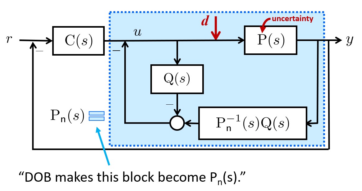
For this post, I’ll introduce simulation results of 4-cart system. If you are not familiar with DOB, please check this post for a comprehensive overview.

Relative degree

Before showing you the problem setting, let’s first grasp the concept of relative degree. If you’ve taken undergraduate control courses, the term relative degree might sound familiar. The relative degree of a system can be determined by examining the degrees of the transfer function’s denominator and numerator.

Relative degree : Degree of the denominator - Degree of the numerator

It is also crucial to grasp the following interpretation:

Relative Degree: The number of derivatives needed to be applied to the output (y) until the input (u) becomes explicitly visible.

Some of you might be unfamiliar with this interpretation, since this concept originated from the nonlinear system theory. However, it is also extremely useful in gaining insights when studying linear systems. Now, let’s move on to the simulation setting.

1. 4-Cart system

Let’s first look at the figure below

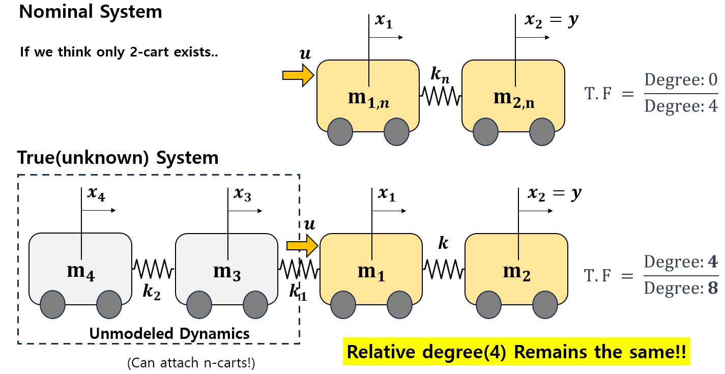
Assume that we have the nominal model consists of two cart(mass) connected by springs. However, the true(unknown) system was actually a 4-cart system. We can apply the force into the $m_1$ cart, and the output y represents the position of the second cart. Let the nominal parameter $k=m_1=m_2=1$. Also let true(unknown) parameter as $m_1=1.05$, $m_2=0.95$, $m_3=1.2$, $k=0.5$, $k_1=0.5$, $k_2=0.5$. Additionally, assume sinusoidal disturbance $d=3 \sin{1.5t}$ is added to the input before feeding it into the true system.

Control Objective : Starting from the origin, move the second cart($y=x_2$) to position $y=1m$ and stabilize the system.

This problem seems to to be extremely challenging because we do not have much information of the true system dynamics(with additional 2-cart attached). Also, we face uncertainties in crucial parameters such as mass and spring constants, which makes the problem even more challenging. Despite this unmodeled dynamics and parametric uncertainties with external disturbances, I’ll show the surprising efficacy of DOB in tackling this complex problem.

To check the applicability of DOB, a critical step involves checking the relative degree of the system, which was mentioned earlier. As highlighted, the relative degree denotes how many derivatives must be applied to the output until the input u becomes explicitly visible. We can easily infer from the diagram that the relatively degree will remain the same between the nominal system and the true system. In our scenario, the consistent relative position of u and y ensures the preservation of the relative degree.

For the readers, let’s re-check whether the relative degree is the same by deriving the transfer functions of both nominal and true systems.

Equation of the nominal system:

• $m_{1,n}\ddot{x}_1 = k_n (y-x_1)+u$
• $m_{2,n}\ddot{y} = k_n (x_1 -y)$

With the above equation, we can derive the transfer function of the nominal system:

• $P_n (s) = \frac{k_n}{ m_{1,n}m_{2,n}s^4 + k_n(m_{1,n}+m_{2,n})s^2 }$ where the relative degree is 4

For the true system,

• $m_4 \ddot{x}_4 = k_2 (x_3-x_4)$
• $m_3 \ddot{x}_3 = k_1 (x_1-x_3)+k_2(x_4-x_3)$
• $m_1 \ddot{x}_1 = u + k(y-x_1) + k_1 (x_3-x_1)$
• $m_2 \ddot{y} = k(x_1-y)$

Obtaining transfer function of this true system are slightly complicated. We finally get the transfer function $P(s)$

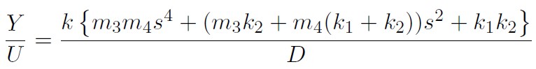where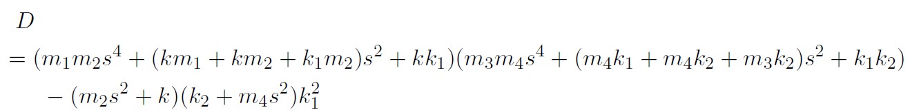

For the true system, Relative degree = 8-4 = 4. We observe that both the true system and the nominal system share the same relative degree of 4.

While in real-world applications, calculating the true transfer function as demonstrated above may not be possible. However, if the “relative position” between input and output remains the same, we can reasonably “claim” that the relative degree remains the same.

As we have established that the relative degree is consistent for this 4-cart system, let’s now see how DOB can be used in this context.

Q-filter

As the relative degree of the system = 4, let’s use the Q-filter with degree=4.

where $a_3=3$, $a_2=3$, $a_1=1$, $a_0=0.2$. If the DOB has been successfully applied, the system will “behave” just like the nominal 2-cart model.

For the nominal 2-cart problem, let’s use basic lead-lag compensator $C(s)=-\frac{6.83s^2-1.84s-0.28}{s^2+4.27s+6.07}$, which was designed using the nominal parameters with 2-cart nominal dynamics.

Now, let’s check the power of the DOB

Simulation result

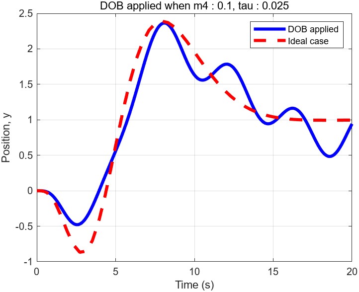
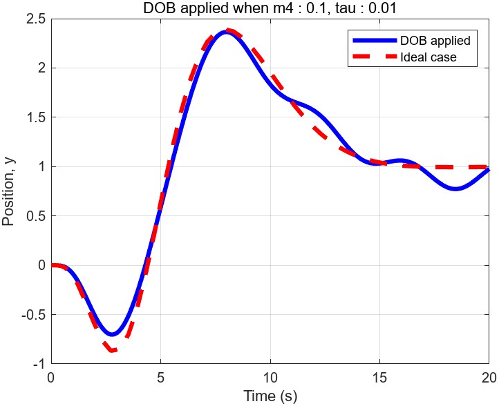
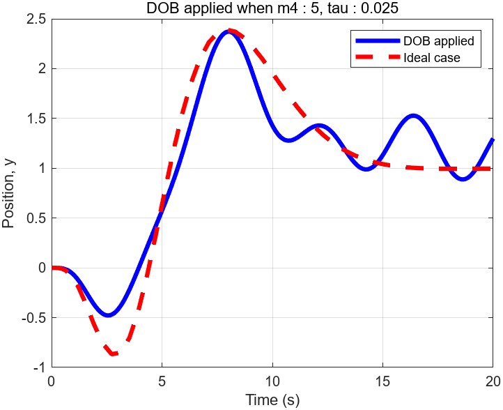
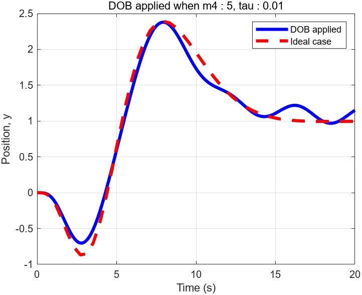
The red line illustrates the output y(position of the second cart) in the ideal scenario when the controller is applied to the nominal system(2-cart). The blue line represents the output y of the true 4-cart system. Notably, the output y is effectively stabilized at the desired position y = 1m. Additionally, you can observe that the blue line is getting closer to the red line with a smaller $\tau=0.01$. It is well-known established fact that the performance of the DOB improves as we decrease $\tau$. However, you need to be careful for choosing excessively small $\tau$ since this can amplify the impact of unmodeled fast-dynamics. In real-world implementations, determining proper $\tau$ and Q-filter coefficients requires a careful process of trial and error.

Conclusion

Throughout this post, I’ve showcased simulation results demonstrating the effectiveness of using DOB to control a 4-cart system with a nominal 2-cart model. The surprising outcome is the stabilization of a system contaminated by parametric uncertainties, unmodeled dynamics, and external disturbances. Imagine you are trying to stabilize a mass-spring cart being unaware of an extra cart attached with unknown parameters and external disturbances. It would be extremely challenging, wouldn’t it?

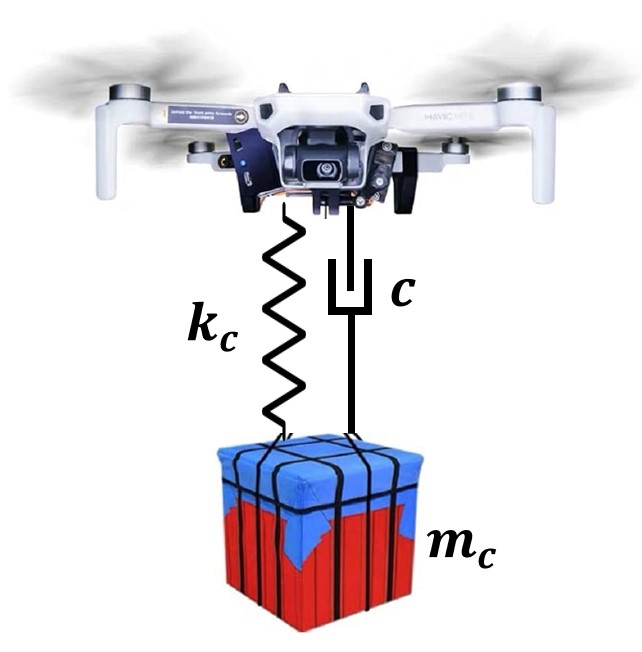
I hope this magic-like-example has captured your interest. In the next post, I’ll dive into more complicated simulation involving quadrotor-delivery dynamics with MPC. Stay tuned for the upcoming post!