DOB+MPC Simulation (Quadrotor Delivery)

DOB + MPC simulation of quadrotor delivery application

In this post, I’ll present simulation results for DOB + MPC(Model Predictive Control), using the quadrotor dynamics. Recently, quadrotors are often used to deliver payloads such as food or medical devices to the rural areas. Various methods such as adaptive control are suggested to handle uncertainties with disturbances to ensure the safety of the system. In this post, we explore the use of DOB as an add-on robust controller in conjunction with MPC.

Why DOB+MPC?

Typically, MPC employs a linear state-space model and optimizes a quadratic cost function for a finite horizon in the future. The quality of the model significantly influences the prediction of the system behavior, especially for real-world MPC performance. To address this challenge, the concept of DOB comes into play, ensuring that the true dynamic model behaves similar to the nominal model. If DOB successfully makes the true system behavior just as the nominal model, it gives confidence in utilizing model-based algorithms like MPC.

Quadrotor Dynamics with mass-spring-damper payload attached

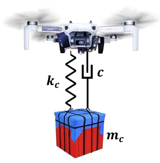
For simplicity, I assumed that the mass-spring-damper payload dynamics only affect the z-dynamics of the quadrotor. Let the state variables of quadrotor dynamics as follows:

• $(x,y,z)$ : Position of the center of the gravity of the quadrotor
• $(z_c)$ : Position of the cargo in z coordinate
• $(\phi, \theta, \psi)$ : Roll, Pitch, Yaw angle of the quadrotor
• $(\dot{x}, \dot{y}, \dot{z})$ : Velocity of the quadrotor for each coordinate in earth-frame
• $(\dot{z}_c)$ : Velocity of the cargo in z coordinate
• $(\dot{\phi}, \dot{\theta}, \dot{\psi})$ : Angular velocity for each coordinate in body-frame

Dynamical model of the quadrotor

The dynamical model of the quadrotor can be written as following equations:

• $\ddot{x} = (\cos\phi \sin\theta \cos \psi + \sin \phi \sin\psi)\frac{U_1}{m}$
• $\ddot{y} = (\cos\phi \sin\theta \sin \psi - \sin \phi \cos\psi)\frac{U_1}{m}$
• $\ddot{z} = -g+(\cos\phi \cos\theta)\frac{U_1}{m} + \frac{c}{m}(\dot{z_c}-\dot{z})-\frac{k_c}{m}(z-z_c)$
• $\ddot{z_c} = -g - \frac{c}{m_c}(\dot{z_c}-\dot{z})+\frac{k_c}{m_c}(z-z_c)$
• $\ddot{\phi} = \dot{\theta}\dot{\psi}(\frac{I_y-I_z}{I_x})+\frac{L}{I_x}U_2$
• $\ddot{\theta} = \dot{\phi}\dot{\psi}(\frac{I_z-I_x}{I_y})+\frac{L}{I_y}U_3$
• $\ddot{\psi} = \dot{\phi}\dot{\theta}(\frac{I_x-I_y}{I_z}) + \frac{1}{I_z}U_4$

where $m$ and $m_c$ is the mass of the quadrotor and the payload each. Also, $k_c$ denotes the spring constant of the payload, and $c$ denotes the damping constant of the equivalent mass-spring-damper system. $I_x, I_y, I_z$ represents the moments of inertia for each coordinate. Note that the mass-spring-damper system of payload was added to the z-dynamics. Here, air drag force and reaction forces from the propeller blades were ignored and treated as disturbances. For the simulation, we utilized the above dynamics as the true dynamics with the unknown parameters.

Simplified Dynamical model of the quadrotor

Since the dynamics are complex and coupled between each other, the well-known decoupling techniques were used to simplify the system. With the small angle approximation, we get the linearized dynamics of the quadrotor as follows:

• $\ddot{x}=g\theta$
• $\ddot{y}= -g\phi$
• $\ddot{z} = -g+ \frac{U_1}{m_n}$
• $\ddot{\phi} =\frac{L_n}{I_{x,n}}U_2$
• $\ddot{\theta} = \frac{L_n}{I_{y,n}}U_3$
• $\ddot{\psi} = \frac{1}{I_{z,n}}U_4$

where index $n$ denotes the nominal parameter we used. Note that our nominal dynamics do not include any information of the payload. Many existing model-based control algorithms, such as Optimal Control, rely on simplified model for controller design. However, the performance of these controllers degrades when the true dynamics of the system deviate from the nominal model. Additionally, it is important to determine whether the simplified dynamics adequately represent the true dynamics. For controller designer, it is important to ensure the controller designed from simplified dynamics will also work well in true system, especially in safety-critical systems, which is typically hard to verify.

The power of DOB becomes apparent in addressing this challenge by ensuring that the true dynamics closely follow the simplified decoupled dynamics. This increases confidence of the control engineer when designing their own controller. In this context, we implement DOB for each state variable $(x,y,z)$ and $(\phi, \theta, \psi)$ to behave as the simplified decoupled model. Also, additional strength of the DOB has emerged while implementation as it also provides the true state variable within the High-gain observer structure. We leveraged this information to design a stabilizing controller using MPC.

Control Objective

1. Starting from $x=y=z=0$, arrive $x=1, y=1, z=4$ while stabilizing the system
2. State of the quadrotor needs to satisfy the following constraints
   • $-0.45\pi \leq \phi, \theta \leq 0.45\pi$
   • $-0.5\pi \leq \psi \leq 0.5\pi$
   • $-10 \leq x,y \leq 10$
   • $0 \leq z \leq 10$
3. The mass-spring-damper payload was attached from the beginning and released at $t=50s$ (payload delivered!). Quadrotor should maintain stability despite the rapid change of the dynamics.

DOB Design

Before designing the DOB Q-filter, let’s analyze the relative degree of the system to determine whether the DOB can effectively handle the unmodeled dynamics from the payload. From the simplified dynamics, we observe that the dynamics of $z, \phi, \theta, \psi$ are double integrators, while the dynamics of $x, y$ are quadruple integrators. In other words, the nominal dynamics of $z, \phi, \theta, \psi$ have a relative degree of 2, while the nominal dynamics of $x$ and $y$ have a relative degree of 4. The former group works as “fast” states, and $x, y$ works as “slow” states.

To design the controller, we decomposed the dynamics into two modules, position($x,y,z$) and attitude($\phi,\theta,\psi$) dynamics. This approach is commonly used in controller design, where the attitude controller stabilizes the angles to follow the desired angles. Also, the position controller provides the attitude controller with the reference angle to reach the desired position at a higher level. Additionally, for the $x$ and $y$ dynamics, $\theta$ and $\psi$ are considered as inputs, allowing all 6 states in simplified dynamics to be regarded as relative degree 2. The nominal dynamics for the attitude controller can be expressed in linear state space as:

$\begin{bmatrix} \dot{\phi} \\ \dot{\theta} \\ \dot{\psi} \\ \ddot{\phi}\\ \ddot{\theta} \\ \ddot{\psi} \end{bmatrix} =\begin{bmatrix} 0 & 0 & 0 & 1 & 0 & 0 \\ 0 & 0 & 0 & 0 & 1 & 0 \\ 0 & 0 & 0 & 0 & 0 & 1 \\ 0 & 0 & 0 & 0 & 0 & 0 \\ 0 & 0 & 0 & 0 & 0 & 0 \\ 0 & 0 & 0 & 0 & 0 & 0 \\ \end{bmatrix} \begin{bmatrix} {\phi} \\ {\theta} \\ {\psi} \\ \dot{\phi} \\ \dot{\theta} \\ \dot{\psi} \end{bmatrix} + \begin{bmatrix} 0 & 0 & 0 \\ 0 & 0 & 0 \\ 0 & 0 & 0 \\ \frac{L_n}{I_{x,n}} & 0 & 0 \\ 0 & \frac{L_n}{I_{y,n}} & 0 \\ 0 & 0 & \frac{1}{I_{z,n}} \end{bmatrix} \begin{bmatrix} U_2 \\ U_3 \\ U_4 \end{bmatrix}$

similarly, the nominal position dynamics can be written as

$\begin{bmatrix} \dot{x} \\ \dot{y} \\ \dot{z} \\ \ddot{x} \\ \ddot{y} \\ \ddot{z} \end{bmatrix} = \begin{bmatrix} 0 & 0 & 0 & 1 & 0 & 0 \\ 0 & 0 & 0 & 0 & 1 & 0 \\ 0 & 0 & 0 & 0 & 0 & 1 \\ 0 & 0 & 0 & 0 & 0 & 0 \\ 0 & 0 & 0 & 0 & 0 & 0 \\ 0 & 0 & 0 & 0 & 0 & 0 \\ \end{bmatrix} \begin{bmatrix} {x} \\ {y} \\ {z} \\ \dot{x} \\ \dot{y} \\ \dot{z} \end{bmatrix} + \begin{bmatrix} 0 & 0 & 0 \\ 0 & 0 & 0 \\ 0 & 0 & 0 \\ g & 0 & 0 \\ 0 & -g & 0 \\ 0 & 0 & \frac{1}{m_n} \end{bmatrix} \begin{bmatrix} \theta \\ \phi \\ {\Delta U}_1 \end{bmatrix}$

Now, for the quadrotor to follow the nominal dynamics we used Q-filter of

$Q(s) := \frac{a_0}{(\tau s)^2 + a_1 (\tau s) + a_0}$

where $a_0=20$, $a_1=10$, and different $\tau$ was implemented to check how $\tau$ effects the control performance. The overall scheme of the quadrotor control is as follows:

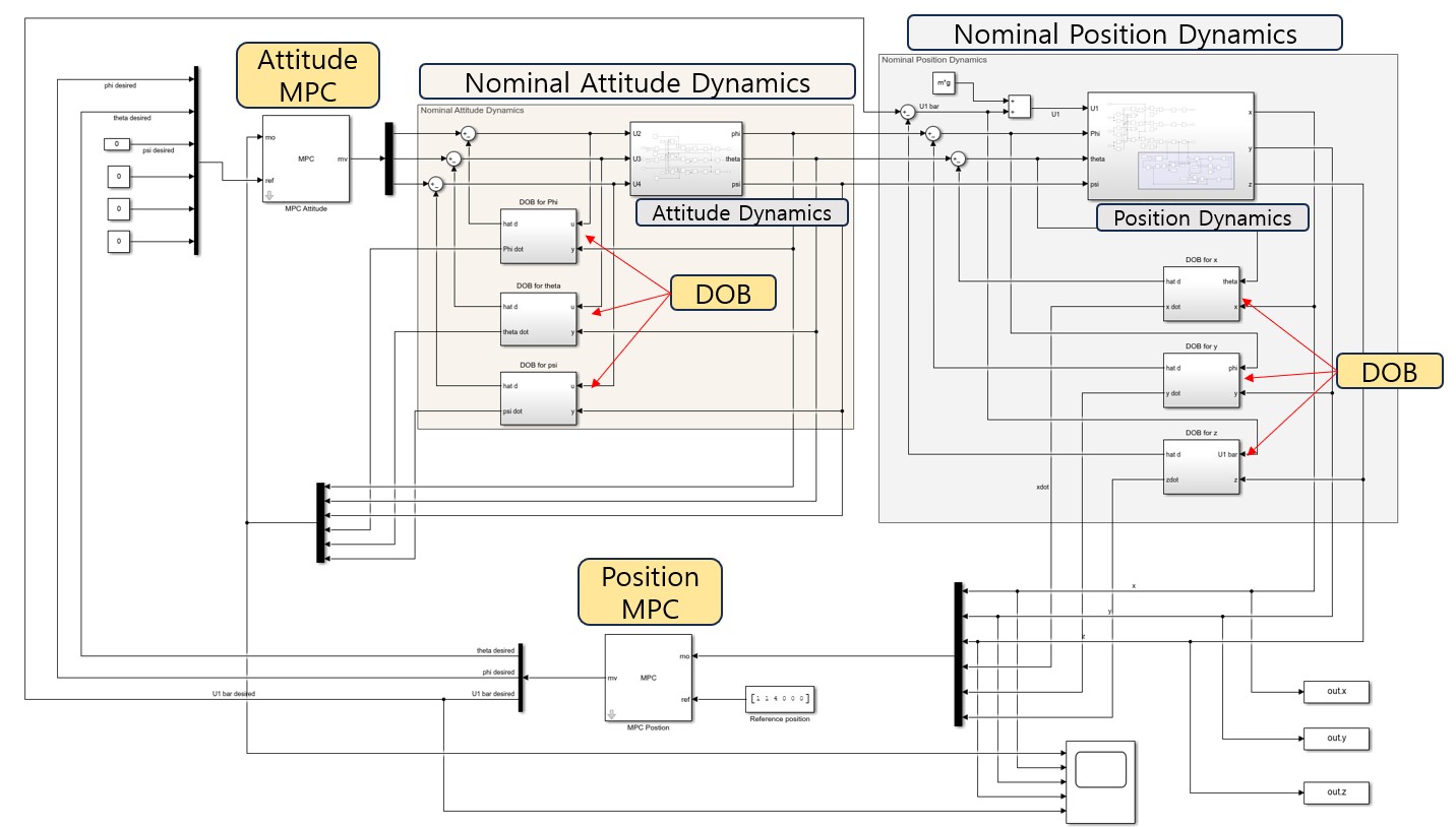
Let’s first focus on the brown box representing the attitude dynamics. The subsystem inside, labeled as ‘Attitude Dynamics’ shows the true dynamical model of the attitude($\phi, \theta, \psi$) with $U_2, U_3, U_4$ as inputs. By incorporating 3 DOBs for each $\phi, \theta$ and $\psi$, the brown box behaves as ‘Nominal Attitude Dynamics’, enabling the design of the Attitude MPC from nominal dynamics without additional concerns. The true attitude dynamics used for the experiment is

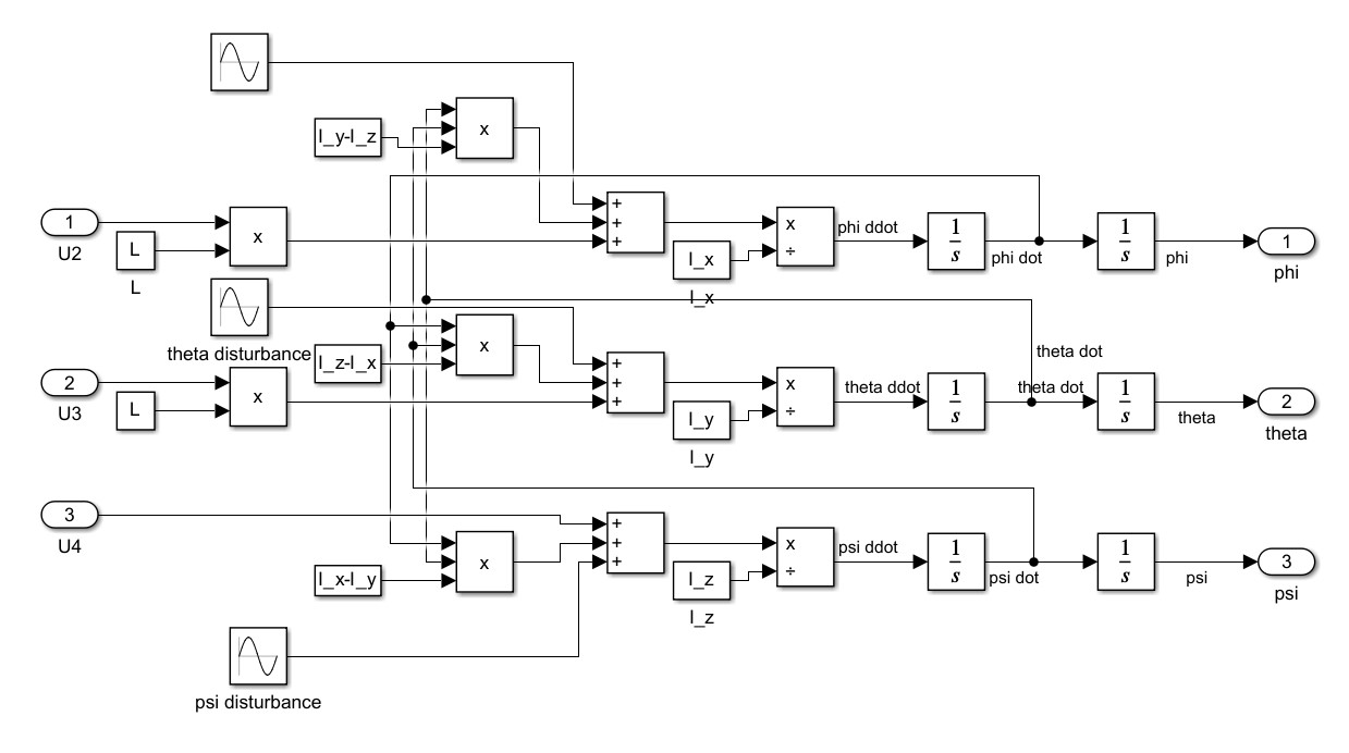
Next, let’s look at the gray box which descibes the Position dynamics. The subsystem inside denoted as ‘Position Dynamics’ is the true dynamical model of the position(x,y,z) with $U_1, \phi, \theta, \psi$ as an input. The true position dynamics is as

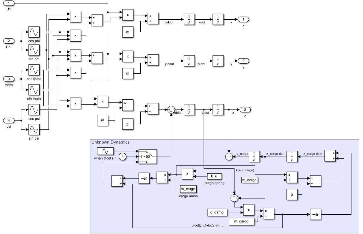
On the bottom of figure, unknown dynamics which describes the payload mass-spring-damper system is attached. Clock block was utilized to express the payload release mission at $t=50s$. 3 DOBs were utilized to make the gray block behaves like nominal position dynamics. Thanks to DOB, we now have two modules that behave like nominal attitude and position dynamics. The following section explains how the outer controller(MPC) was designed for the given mission.

MPC design

While there is some freedom in choosing controllers, we used MPC for both the Position and Attitude controllers for the following reasons.

• Dynamics can be treated as linear, thanks to the power of DOB.
• MPC can explicitly handle constraints. Given the strict constraints on all state variables in our system, tuning classic controllers (e.g., PID) to meet these control constraints is challenging.
• Tuning the gain parameter is relatively straightforward.

By utilizing MPC Toolbox in MATLAB, we can easily tune the gain parameters and immediately evaluate the results. However, despite the strict constraints, the tuning process took several hours to meet the given task. Throughout this section, I will share some insights gained from this process (without any justification!!)

• The sampling frequency needs to be fast enough to handle fast variables. In the case of this quadrotor task, the MPC for attitude dynamics must be sampled faster than the position dynamics. MPC for position dynamics works as a higher-level decision maker and provides the attitude angle to the Attitdue MPC as a reference. The mission of the Attitude MPC is to ensure the attitude angle follows the given reference angle. To achieve this, the sampling frequency of attitude MPC needs to be fast enough as it acts as a lower-level controller.
• With the appropriate sampling frequency, setting a proper horizon length is crucial to achieve the goal. The horizon length should be selected long enough to understand events in the time scale. For example, the higher-level controller(Position MPC in this case) must have the ability to look forward into the long future. Even if a high sampling frequency isn’t used, at least the horizon length must be selected long enough. The goal of the low-level controller(Attitude MPC) is to quickly follow the reference attitude angle; it doesn’t have to look far into the future, but should utilize computation resources for a higher sampling frequency.

As a result, the sampling frequency for Attitude MPC was selected as $(50Hz=1/0.02s)$ with the horizon length of $200(0.02s\times200=4s)$. The sampling frequency for Position MPC was selected as $(10Hz=1/0.1s)$ with the horizon length of $200(0.1s\times200=20s)$. For the gain parameter, parameters for reference variables were selected as large values. The following section shows the experiment results by utilizing the suggested controllers.

Simulation Results

For the true parameters, $m=0.76 kg$, $L=0.14m$, $I_x = 0.0045 kg\cdot m^2$, $I_y = 0.0045 kg\cdot m^2$, $I_z = 0.0113 kg\cdot m^2$, $k_c=0.5 N/m$, $m_c = 5 kg$, $c=0.5 kg/s$ were used. For the nominal parameters, $m_n=0.6 kg$, $L_n=0.15m$, $I_{x,n} = 0.005 kg\cdot m^2$, $I_{y,n} = 0.005 kg\cdot m^2$, $I_{z,n} = 0.012 kg\cdot m^2$ were used.

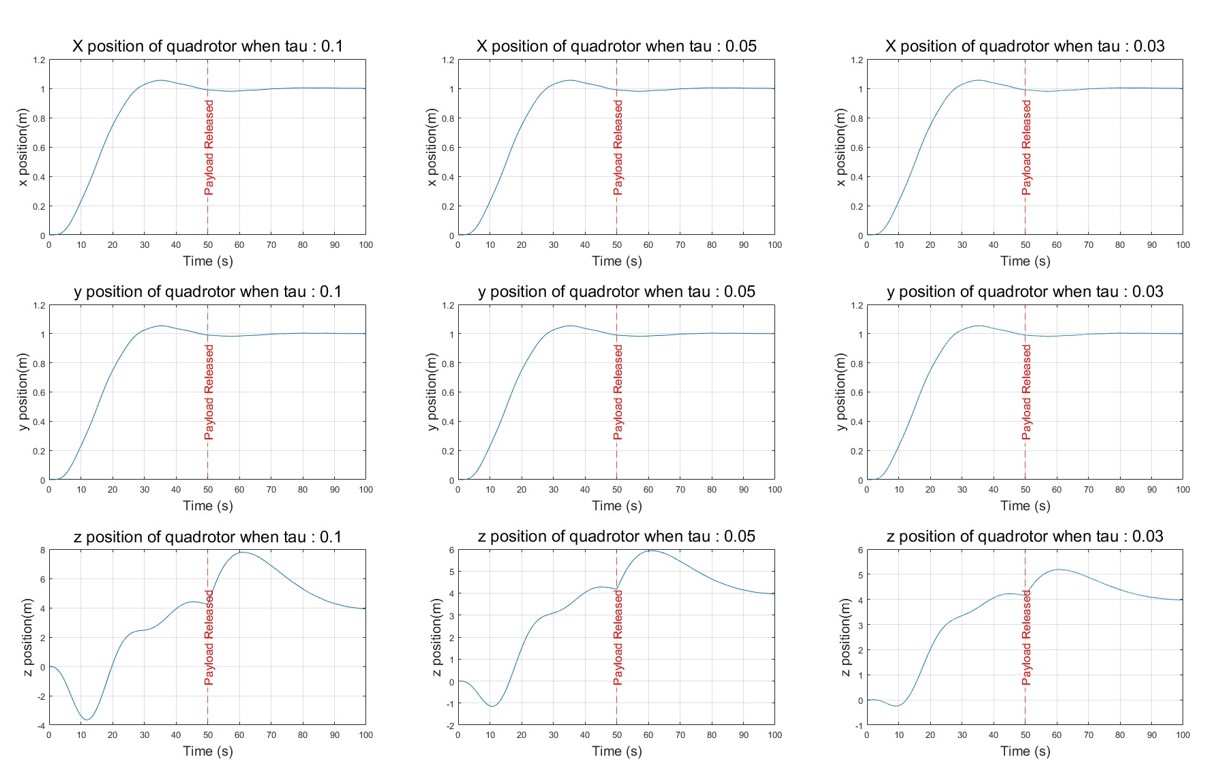
The above figure shows the x,y,z position of the quadrotor when $\tau=0.1,0.05,0.03$. The positions of $x$ and $y$ smoothly reach the desired positions, while the z-position exhibits some undershoot with undesired movements. Nevertheless, it approximately converges to the target position $z=4m$. At $t=50s$, the payload was released, causing the quadrotor’s z-position to move upward as the gravitational force from the payload suddenly disappeared. As $\tau$ becomes smaller, z-position displays less overshoot/undershoot behavior.

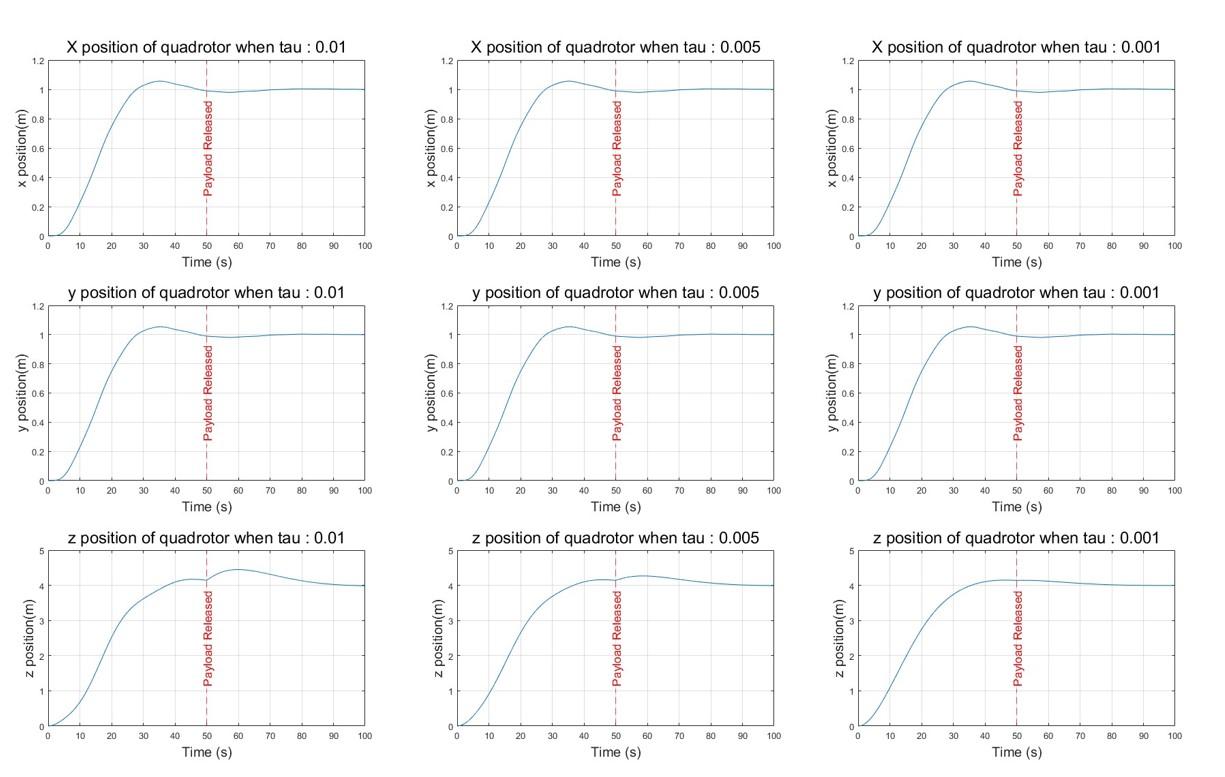
The above figure shows the x,y,z positions of the quadrotor are shown for $\tau=0.01,0.005,0.001$. The positions of $x$ and $y$ exhibit desirable behavior toward the goal position. The undershoot problem of z-position is fixed as the $\tau$ becomes smaller. Also, the effect of payload release at $t=50s$ is nearly eliminated when $\tau=0.001$.

Animation

For 3D visualization of the simulation results, I used Matlab Drone Animation from Jitendra singh.

When $\tau=0.1$, you can see the big flucuation in z-direction. Also, in the middle of the animation, quadrotor rapidly ascends as it releases the payload at $t=50s$.

When $\tau=0.05$, the movement is smoother compared to $\tau=0.1$, but it still shows significant fluctuations.

When $\tau=0.005$, you can observe smooth movement despite the presence of payload dynamics.

When $\tau=0.001$, the majority of the fluctuating movement was eliminated, almost as if nothing was attached!

As $\tau$ decreases, the fluctuation reduces, and the impact of the unmodeled payload dynamics becomes smaller!

Conclusion

In conclusion, we’ve seen that MPC+DOB controller has stabilized the quadrotor system despite of the unknown parameters with unmodeled payload dynamics. In the outloop controller, two MPCs were employed to handle nominal dynamics, with DOB taking on the responsibility of ensuring the system behave like the nominal system. Simulation results demonstrated the success of the proposed method in achieving the assigned task, with performance improving as $\tau$ decreased. Also, the quadrotor was able to stabilize the system after the payload was released, which indicates the sudden change of the z-dynamics. This shows the capabilities of this method to handle unmodeled dynamics when the relative degree remains the same.

This post was quite complicated, but I hope you felt the power of DOB through this post. Stay tuned for the upcoming post!